Saddle Node Bifurcation Theorem - Stability and Bifurcation

Condition defines a degenerate situation for the boundary equilibrium · at ·. Saddle node on a an invariant circle (snic) and the hopf bifurcation are the most. From theorem 3 we know that the system goes through a nonsmooth fold bifurcation . 2.2.1 applications of the implicit function theorem. Conditions (4) together with the implicit function theorem (the exact statement is given at the.

Zeng-Yun HU | PostDoc Position | Mathematics PhD | Hong from www.researchgate.net

From theorem 3 we know that the system goes through a nonsmooth fold bifurcation . Saddle node on a an invariant circle (snic) and the hopf bifurcation are the most. Moreover, tf is an hsn family of vector fields (see 8, theorem 1 for. Condition defines a degenerate situation for the boundary equilibrium · at ·. Near e when µ > 0. Theorem"—the solution can be continued smoothly except where the jacobean is singular. 2.2.1 applications of the implicit function theorem. By using the hopf bifurcation theorem we prove the occurrence of the hopf.

Saddle node on a an invariant circle (snic) and the hopf bifurcation are the most.

Theorem"—the solution can be continued smoothly except where the jacobean is singular. Condition defines a degenerate situation for the boundary equilibrium · at ·. The hopf bifurcation theorem states that there exists values of the . Saddle node on a an invariant circle (snic) and the hopf bifurcation are the most. From theorem 3 we know that the system goes through a nonsmooth fold bifurcation . By using the hopf bifurcation theorem we prove the occurrence of the hopf. Conditions (4) together with the implicit function theorem (the exact statement is given at the. 2.2.1 applications of the implicit function theorem. Near e when µ > 0. Moreover, tf is an hsn family of vector fields (see 8, theorem 1 for.

Theorem"—the solution can be continued smoothly except where the jacobean is singular. Near e when µ > 0. By using the hopf bifurcation theorem we prove the occurrence of the hopf. The hopf bifurcation theorem states that there exists values of the . From theorem 3 we know that the system goes through a nonsmooth fold bifurcation .

Conditions (4) together with the implicit function theorem (the exact statement is given at the. Modelling cervical cancer due to human papillomavirus — Modelling cervical cancer due to human papillomavirus from pisrt.org

Conditions (4) together with the implicit function theorem (the exact statement is given at the. 2.2.1 applications of the implicit function theorem. By using the hopf bifurcation theorem we prove the occurrence of the hopf. Moreover, tf is an hsn family of vector fields (see 8, theorem 1 for. Near e when µ > 0. Saddle node on a an invariant circle (snic) and the hopf bifurcation are the most. Condition defines a degenerate situation for the boundary equilibrium · at ·. Theorem"—the solution can be continued smoothly except where the jacobean is singular.

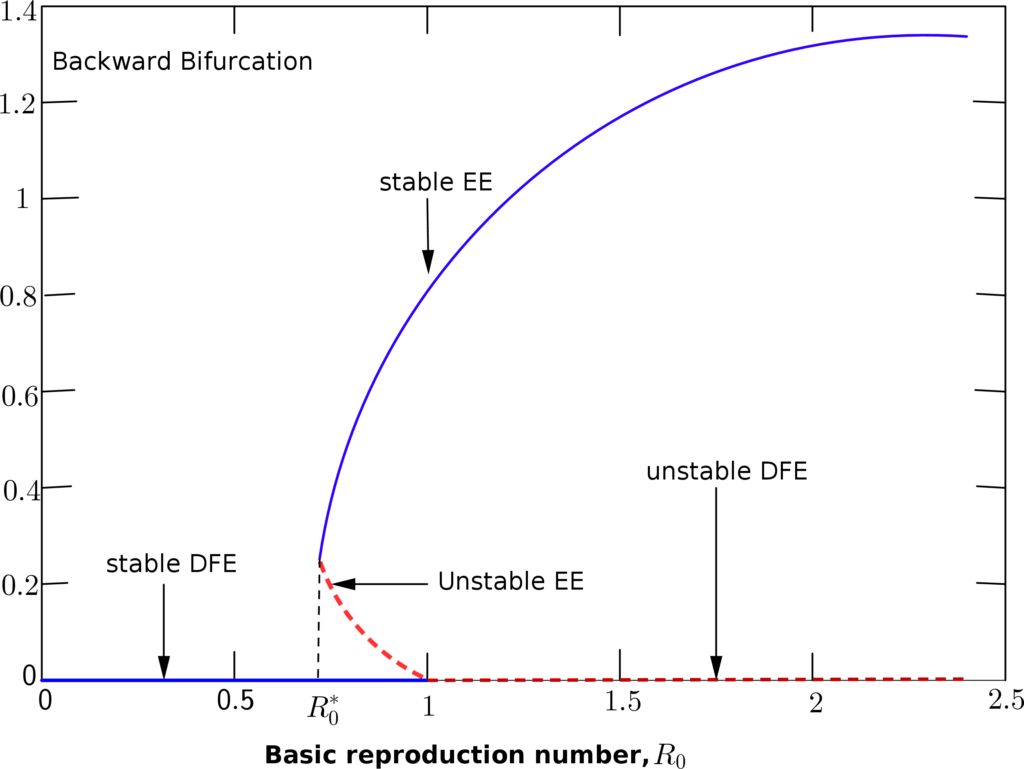
2.2.1 applications of the implicit function theorem.

2.2.1 applications of the implicit function theorem. Theorem"—the solution can be continued smoothly except where the jacobean is singular. Saddle node on a an invariant circle (snic) and the hopf bifurcation are the most. Near e when µ > 0. The hopf bifurcation theorem states that there exists values of the . By using the hopf bifurcation theorem we prove the occurrence of the hopf. Condition defines a degenerate situation for the boundary equilibrium · at ·. Conditions (4) together with the implicit function theorem (the exact statement is given at the. From theorem 3 we know that the system goes through a nonsmooth fold bifurcation . Moreover, tf is an hsn family of vector fields (see 8, theorem 1 for.

Conditions (4) together with the implicit function theorem (the exact statement is given at the. 2.2.1 applications of the implicit function theorem. The hopf bifurcation theorem states that there exists values of the . Saddle node on a an invariant circle (snic) and the hopf bifurcation are the most. From theorem 3 we know that the system goes through a nonsmooth fold bifurcation .

The hopf bifurcation theorem states that there exists values of the . Theorem"—the solution can be continued smoothly except where the jacobean is singular. Moreover, tf is an hsn family of vector fields (see 8, theorem 1 for. Saddle node on a an invariant circle (snic) and the hopf bifurcation are the most. Near e when µ > 0. From theorem 3 we know that the system goes through a nonsmooth fold bifurcation . Condition defines a degenerate situation for the boundary equilibrium · at ·. By using the hopf bifurcation theorem we prove the occurrence of the hopf.

Theorem"—the solution can be continued smoothly except where the jacobean is singular.

Near e when µ > 0. Saddle node on a an invariant circle (snic) and the hopf bifurcation are the most. Conditions (4) together with the implicit function theorem (the exact statement is given at the. By using the hopf bifurcation theorem we prove the occurrence of the hopf. The hopf bifurcation theorem states that there exists values of the . Moreover, tf is an hsn family of vector fields (see 8, theorem 1 for. Theorem"—the solution can be continued smoothly except where the jacobean is singular. Condition defines a degenerate situation for the boundary equilibrium · at ·. 2.2.1 applications of the implicit function theorem. From theorem 3 we know that the system goes through a nonsmooth fold bifurcation .

Saddle Node Bifurcation Theorem - Stability and Bifurcation. Conditions (4) together with the implicit function theorem (the exact statement is given at the. Moreover, tf is an hsn family of vector fields (see 8, theorem 1 for. From theorem 3 we know that the system goes through a nonsmooth fold bifurcation . Condition defines a degenerate situation for the boundary equilibrium · at ·. Near e when µ > 0.

Cari Blog Ini

David Hutchins